

virgin =SUM() users vs chad click at each cell enjoyers
What is even happening here? There is a sum of like every 13th cell?
My guess is that there are multiple tables on one sheet, and this is the summation of the sub-totals.
Multiple things formatted to look like tables, but not actually tables. And they are summing like every 13th cell. It is wild over here.
Every 13 cells could be summing the total of multiple years of data. Eg 12 month + 1 total, rinse and repeat. Then summing just the total cells for each year. 💁
I guess this is Excel.
Wait, that’s an actual formula. When I first saw this I thought it was an employee going insane and keysmashing into a spreadsheet as evidenced by the “send help”.
Yup, actual formula. Might not even be the most offensive one in the spreadsheet.
Wait till AI is able to help.
=TEXTJOIN("",TRUE,A330,A443,A556,A669,A782,A895,A1008,A1121,A1234,A1347,A1460,A1573,A1686,A1799,A2112,A2225,A2338,A2451,A2564,A2677,A2790,A3303,A3316,A3329,A3342,A3355,A3368,A3381,A3394,A5407,A5420,A5433,A5446,A5459,A5472,A5485,A5498,A5511,A5524,A5537,A5550,A5563,A5576,A5589,A5602,A5615,A5628,A5641,A5654,A5667)OMG. Which AI tool produced this?
Claude. To be fair, it had trouble OCR-ing it. After way too much back and forth about the pattern, it produced this:
=LET(
    rows, SEQUENCE(INT((667-30)/13+1),1,30,13),
    SUM(INDEX(AA:AA,rows))
)
Which is correct, but obviously the calculations would be best served by reorganizing the table and probably using a pivot table or at least grouping and subtotaling.
I must find the monstrous function which indexes virtual arrays that I implemented in a Google sheet of mine when I discovered there’s no limit to how reckless you can be in a single cell.
Edit: Here it is:
ARRAYFORMULA(IFERROR((INDEX('Invoice History'!$A$7:$A$44, SMALL(IF(($G$3='Invoice History'!$D$7:$D$44)*('Invoice History'!$F$7:$F$44="Unpaid"), MATCH(ROW('Invoice History'!$A$7:$A$44), ROW('Invoice History'!$A$7:$A$44)), ""), ROW(A1))))))According to my documentation, it is used for “Looking up a value on a row, on another sheet, where two other values on that row match the given criteria”
Resume: “Experienced Excel Wizard”
I have written similarly awful formulae when I needed to get a csv to export to Google Calendars, but the program I was exporting to wasn’t using Google’s accepted csv headers.
I ended up creating a template that looked at the exported csv file, and then reformatted it in a way that Google liked (and added some extra info along the way.) I needed it to only fill text if an entry actually had info in it, and hide all the text otherwise. So that I could automatically delete empty cells and avoid a bunch of empty calendar entries when importing it into Google. The resulting formula for some of the fields was… Not great. This is what controlled the “name” of each calendar event:
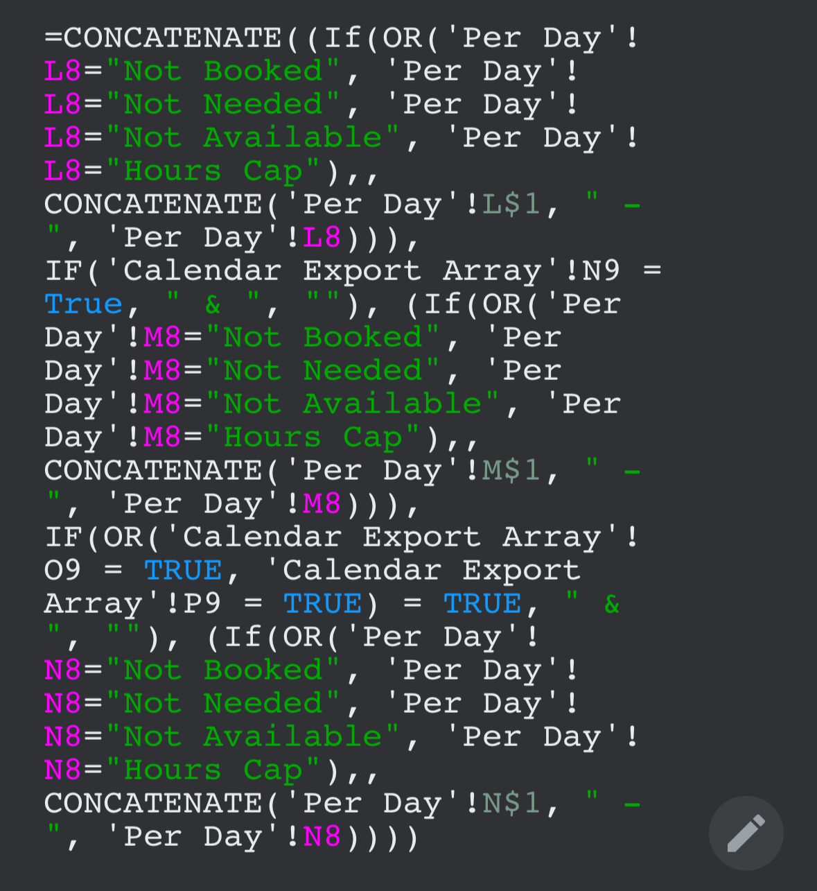
It takes several different potential fields, and combines them into a single field. If there are no entries, it gets left blank.
And every single time I would get it working properly, someone would add a row or change the data validation rules, so I would have to go in and update my formulae. After the fifth or sixth time that happened, I told the person making the changes that it was his job to update the formulae. Suddenly, it stopped getting changed.
That’s bonkers but I can follow it, I think. Good work!
Damn. At that point I would just switch over to a macro. Although I also have some formulas that xlookup a value, concatenate it, and the xlookup the new concatenated value.
I winced.


